Logistic Regression & classification metrics

import matplotlib.pyplot as plt
import numpy as np
import pandas as pd
from sklearn.datasets import load_breast_cancer
from sklearn.linear_model import LogisticRegression
from sklearn.metrics import accuracy_score
from sklearn.metrics import precision_score
from sklearn.metrics import recall_score
from sklearn.metrics import f1_score
from sklearn.metrics import roc_auc_score
from sklearn.metrics import average_precision_score
from sklearn.metrics import confusion_matrix
from sklearn.model_selection import train_test_split
from sklearn.preprocessing import StandardScaler

Sigmoid function

先簡單用圖形看一下 sigmoid function 與 logit 的關係。

看當我們使用 a + b * x 去 fit logit時，改變 a 的值，和改變 b 的值，分別對sigmoid function有什麼影響。

def sigmoid(logit: np.ndarray) -> np.ndarray:
    """
    convert logit to probability

    Args:
        logit: A scalar, numpy array of any size.

    Returns:
        p: probability, with the same shape as logit
    """

    p = 1/(1+np.exp(-logit))

    return p

def logit(a, b, x):

    return a + b * x

a 的影響

利用numpy的linspace生成-10到10之間的300個資料點：

x = np.linspace(-10, 10, 300)

# Plot the sigmoid function
plt.figure()

# Set ggplot style
plt.style.use('ggplot')

b = 1
for a in [-1, 0, 1]:
    plt.plot(x, sigmoid(logit(a=a, b=b, x=x)), marker='o', label=f'a={a}')

# Set labels and title
plt.title("Sigmoid Plot")
plt.xlabel("x")
plt.ylabel("sigmoid(a + bx)")

# Show legend
plt.legend()

# Show plot
plt.grid(True)
plt.show()

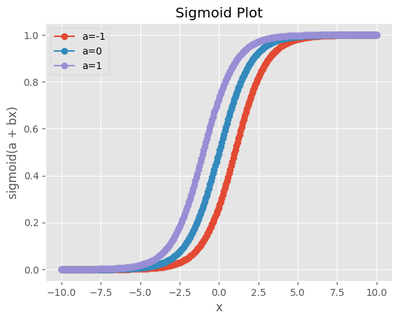
可以注意到 a 的影響是會讓sigmoid function左右移動。

在這個例子中，當預測分類的門檻 = 0.5，若 a < 0，x的取值要大於0才會輸出預測分類為1；反之，若 a > 0 ，x的取值要小於0才會輸出預測分類為1。

b 的影響

同樣生成300個資料點：

x = np.linspace(-10, 10, 300)

# Plot the sigmoid function
plt.figure()

# Set ggplot style
plt.style.use('ggplot')

a = 0
for b in [-0.1, 0.3, 0.5, 1]:
    plt.plot(x, sigmoid(logit(a=a, b=b, x=x)), marker='o', label=f'b={b}')

# Set labels and title
plt.title("Sigmoid Plot")
plt.xlabel("x")
plt.ylabel("sigmoid(a + bx)")

# Show legend
plt.legend()

# Show plot
plt.grid(True)
plt.show()

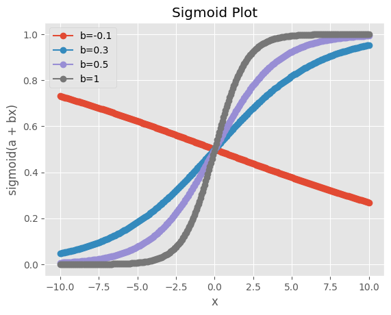
可以看到 b 會影響 sigmoid function S型的曲度。

在這個例子中，當 x 接近0時，b 越大，輸出機率的變化越大。

Logistic Regression for classification

本次使用scikit-learn 的 breast cancer dataset。

該資料集的target紀錄的是腫瘤的分類，target=1為惡性(malignant)，target=0代表良性(benign)。

因此是一個分類問題，我們先用logistic regression來訓練看看。

首先一樣需讀入資料集。

# Load the breast cancer dataset
cancer = load_breast_cancer()
X, y = cancer.data, cancer.target

觀察一下資料集發現feature有尺度差距過大的問題，這樣在做gradient descent的時候會比較沒有效率。

所以應該要做feature scaling。

X.mean(axis=0)

array([1.41272917e+01, 1.92896485e+01, 9.19690334e+01, 6.54889104e+02,
       9.63602812e-02, 1.04340984e-01, 8.87993158e-02, 4.89191459e-02,
       1.81161863e-01, 6.27976098e-02, 4.05172056e-01, 1.21685343e+00,
       2.86605923e+00, 4.03370791e+01, 7.04097891e-03, 2.54781388e-02,
       3.18937163e-02, 1.17961371e-02, 2.05422988e-02, 3.79490387e-03,
       1.62691898e+01, 2.56772232e+01, 1.07261213e+02, 8.80583128e+02,
       1.32368594e-01, 2.54265044e-01, 2.72188483e-01, 1.14606223e-01,
       2.90075571e-01, 8.39458172e-02])

特別要注意的是，feature scaling必須在切割資料集之後才能執行。

否則部分testing data的資訊會洩漏到training dataset之中。

X_train, X_test, y_train, y_test = train_test_split(X, y, test_size=0.2, random_state=42)

借助scikit-learn的StandardScaler來做特徵的標準化。

首先需要先初始化建立一個StandardScaler物件。

注意我們是對training data做.fit_transform()，但對testing data是做.transform()。

.fit_transform()代表同時做了 fit + transform 的動作，在這邊的意思是scaler物件會從資料中取得各特徵的平均值與標準差(fit)，然後才做標準化(transform)。

.transform()，則是只做transform，在這邊的意思是利用scaler從training data中fit好的平均值與標準差來進行標準化。

scaler = StandardScaler()

X_train_scaled = scaler.fit_transform(X_train)
X_test_scaled = scaler.transform(X_test)

建立logistic regression，方法跟之前的做法都很像。

# Initialize logistic regression model
logreg = LogisticRegression()

# Train the model on the scaled training data
logreg.fit(X_train_scaled, y_train)

LogisticRegression()

In a Jupyter environment, please rerun this cell to show the HTML representation or trust the notebook.
On GitHub, the HTML representation is unable to render, please try loading this page with nbviewer.org.

使用testing data進行預測，檢驗模型表現。

# Predictions on the test set
y_pred = logreg.predict(X_test_scaled)

這邊輸出的是預測的分類，0代表預測為良性腫瘤，1代表預測為惡性腫瘤。分類的門檻預設就是0.5。

y_pred

array([1, 0, 0, 1, 1, 0, 0, 0, 1, 1, 1, 0, 1, 0, 1, 0, 1, 1, 1, 0, 1, 1,
       0, 1, 1, 1, 1, 1, 1, 0, 1, 1, 1, 1, 1, 1, 0, 1, 0, 1, 1, 0, 1, 1,
       1, 1, 1, 1, 1, 1, 0, 0, 1, 1, 1, 1, 1, 0, 0, 1, 1, 0, 0, 1, 1, 1,
       0, 0, 1, 1, 0, 0, 1, 0, 1, 1, 1, 1, 1, 1, 0, 1, 0, 0, 0, 0, 0, 0,
       1, 1, 1, 1, 1, 1, 1, 1, 0, 0, 1, 0, 0, 1, 0, 0, 1, 1, 1, 0, 1, 1,
       0, 1, 0, 0])

可以利用scikit-learn的confusion_matrix()計算confusion matrix。

# Generate the confusion matrix
cm = confusion_matrix(y_test, y_pred)

# Convert the confusion matrix array into a pandas DataFrame
cm_df = pd.DataFrame(cm.T, index=['Predicted 0', 'Predicted 1'], columns=['Actual 0', 'Actual 1'])

# Display the confusion matrix as a table
print("Confusion Matrix:")
print(cm_df)

Confusion Matrix:
             Actual 0  Actual 1
Predicted 0        41         1
Predicted 1         2        70

一樣借助scikit-learn就可以計算各種分類問題的衡量指標。

# Calculate accuracy
accuracy = accuracy_score(y_test, y_pred)

# Calculate precision
precision = precision_score(y_test, y_pred)

# Calculate recall
recall = recall_score(y_test, y_pred)

# Calculate F1 score
f1 = f1_score(y_test, y_pred)

# Print metrics
print("Accuracy:", accuracy)
print("Precision:", precision)
print("Recall:", recall)
print("F1 Score:", f1)

Accuracy: 0.9736842105263158
Precision: 0.9722222222222222
Recall: 0.9859154929577465
F1 Score: 0.9790209790209791

可以自行手動進行驗算。

# ravel 可以把np.ndarray攤平
tn, fp, fn, tp = cm.ravel()

print('accuracy:', (tn + tp) / cm.sum())
print('precision:', tp / (tp + fp))
print('recall:', tp / (tp + fn))

accuracy: 0.9736842105263158
precision: 0.9722222222222222
recall: 0.9859154929577465

若要計算AUCROC以及AUCPR，必須要有預測機率。

所以這邊利用.predict_proba()方法來進行預測。

注意到，使用.predict_proba()會分別輸出分類為0的預測機率，以及分類為1的預測機率。所以必須取第二欄。

# Assuming logreg is your logistic regression model
y_score = logreg.predict_proba(X_test_scaled)[:, 1]  # Probability of positive class

計算 AUCROC 以及 AUCPR 。

# Calculate AUCROC
auc_roc = roc_auc_score(y_test, y_score)  # y_score should be the predicted probabilities or decision function scores

# Calculate AUCPR
auc_pr = average_precision_score(y_test, y_score)  # y_score should be the predicted probabilities or decision function scores

# Print metrics
print("AUCROC:", auc_roc)
print("AUCPR:", auc_pr)

AUCROC: 0.99737962659679
AUCPR: 0.9983796759737475